Every article about route optimization covers the same short list of algorithm names. Genetic algorithms. Simulated annealing. Ant colony optimization. The list arrives, the names sound impressive, and the reader learns almost nothing about when to use any of them or why one would outperform another on a specific delivery operation.
The reason these articles are shallow is that the interesting part of route optimization techniques is not which algorithm you choose. It is which problem formulation you apply to your operation. Choose the wrong formulation and the best algorithm in the world gives you an optimal solution to the wrong problem. Choose the right formulation and even a basic heuristic produces routes that outperform what experienced dispatchers plan manually.
This guide starts from the mathematics and works forward to the operational decisions. By the end, you will have a clear picture of which route optimization technique applies to which delivery operation, why the choice matters, and what real-world deployments have demonstrated.
The Problem Route Optimization Is Actually Solving
Route optimization techniques reduce to two foundational problems in combinatorial mathematics, both of which have been studied intensively since the 1930s.
The Travelling Salesman Problem
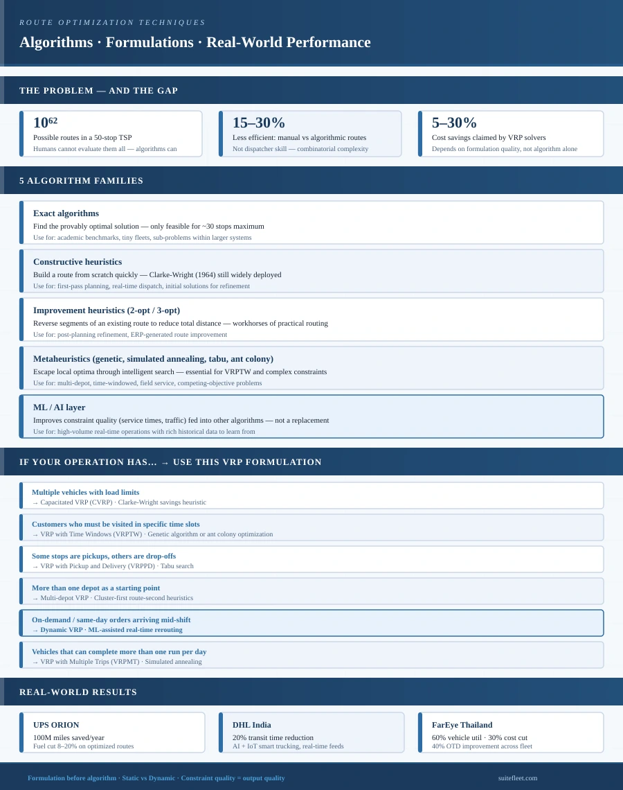
The Travelling Salesman Problem (TSP), first formulated mathematically around 1930, asks a deceptively simple question: given a set of locations, what is the shortest route that visits each one exactly once and returns to the starting point? The problem is classified as NP-hard, meaning that for any problem of non-trivial size, there is no known algorithm that guarantees finding the perfect answer in reasonable time. A 50-location TSP has approximately 10 to the power of 62 possible routes. Evaluating them all, even with the fastest computers, is not feasible.
The Vehicle Routing Problem
The Vehicle Routing Problem (VRP), introduced by George Dantzig and John Ramser in 1959 in the context of fuel delivery optimization, extends the TSP to cover multiple vehicles operating from a depot, each with real-world constraints like load capacity and time-based restrictions. Where TSP concerns one driver visiting all locations, VRP coordinates an entire fleet. The mathematical complexity increases exponentially: a 50-location VRP with 5 vehicles generates a solution space vastly larger than the equivalent TSP. Academic research has identified over 23 distinct VRP variants, each addressing a specific operational constraint.
Commercial VRP routing tools typically claim cost savings of 5 to 30 percent over unoptimized operations. The research consistently shows that skilled human dispatchers create routes that are 15 to 30 percent less efficient than algorithmic solutions. The gap is not because dispatchers are bad at their jobs. It is because the combinatorial space is too large for human intuition to navigate reliably at scale.
If your dispatch team is creating routes manually, the question is not whether optimization would improve things. It is by how much — and the answer depends almost entirely on which formulation you apply, not which algorithm you choose to solve it.
Why the Formulation Matters More Than the Algorithm
Most conversations about route optimization techniques skip directly to algorithms. This is the wrong starting point. Before choosing an algorithm, you need to define exactly what problem you are asking it to solve. That definition is the formulation, and it determines everything that follows.
Consider a beverage distributor running 12 vehicles from a single depot, making daily stops at retailers. The problem is a Capacitated VRP: multiple vehicles, each with a load limit, stops from a single depot, minimize total distance. Any decent CVRP solver produces good routes.
Add the constraint that each retailer has a delivery window during which they accept shipments. The problem becomes a VRP with Time Windows (VRPTW). The solution space is dramatically more complex. The algorithm that worked for the CVRP may now produce routes that look efficient on paper but violate time windows in the field.
Add driver shift lengths, vehicle-specific load types, and different service durations at different stop types — and you are now in the territory of what researchers call the Rich VRP, a problem so constrained that exact solutions are computationally infeasible and metaheuristics become necessary.
A platform that cannot express your constraints in its problem model cannot optimize your operation — regardless of what the algorithm marketing says.
Before evaluating any route optimization vendor, write down the constraints your operation actually has: different vehicle capacities, customer time windows, driver shift limits, vehicle type restrictions, multi-depot structure. Each constraint you identify narrows the set of appropriate formulations. If a platform cannot model all of them, the routes it generates are optimal for a simplified version of your problem — not the one you actually run.
Choosing the Right VRP Formulation for Your Operation
The table below is framed as a decision tool, not an academic taxonomy. Match your operational reality in the left column to find the formulation your optimization system needs to support.
The most common evaluation mistake: selecting a platform based on algorithm quality without verifying whether it can express the correct VRP variant. A CVRP solver applied to a VRPTW operation ignores time windows entirely — or treats them as soft suggestions. Neither is acceptable.
The Five Algorithm Families
With the formulation established, the algorithm choice is a question of trade-offs between solution quality, computational speed, and implementation complexity.
In practice, commercial route optimization systems layer multiple families. A constructive heuristic builds the initial solution. An improvement heuristic refines it. A metaheuristic escapes local optima if time allows. An ML layer adjusts constraint estimates based on historical data. The visible product is one optimized route plan; the underlying process is a pipeline of complementary techniques.
When a vendor says their platform ‘uses AI’ for routing, ask which layer. AI applied to constraint estimation is materially different from AI replacing the optimization algorithm itself. Most ‘AI routing’ is the former — and that is still valuable, but it is not what the marketing implies.
Eight Route Optimization Techniques Explained Operationally
The algorithm names that appear in most articles deserve a more operational description than they typically receive. Here is what each route optimization technique actually does in a delivery context.
Dijkstra's Algorithm — Navigation Layer, Not Route Planning
Dijkstra's algorithm finds the shortest path between two specific points in a road network. It is used inside routing engines at the segment level: calculating travel time from stop A to stop B. It is not a route planner on its own.
If a vendor describes their system as using Dijkstra's algorithm, they are describing the navigation component, not the optimization layer. Every serious routing system uses Dijkstra or a variant (A*, bidirectional Dijkstra) internally. It is infrastructure, not a differentiator.
Nearest Neighbor — Fast Starting Point, Never a Final Answer
Start at the depot, go to the closest unvisited stop, then go to the closest unvisited stop from there, and repeat. Fast, requires almost no computation — and reliably produces routes that are 20 to 25 percent longer than optimal on average.
Nearest neighbor is not a final solution. It is a starting point for improvement algorithms. Its value is speed: generating a baseline that local search methods then refine. Any system offering only nearest-neighbor routing is offering 1960s technology.
Clarke-Wright Savings Algorithm — The Practical Workhorse
Introduced by Geoff Clarke and John Wright in 1964, the savings algorithm starts from the least efficient configuration: one vehicle per customer. It then calculates the saving achieved by merging any two individual routes into one combined route, and merges the highest-saving pairs first, subject to capacity constraints.
The savings algorithm remains in widespread use in commercial systems because it is computationally efficient, naturally respects capacity constraints, and typically produces solutions within 10 to 15 percent of optimal for CVRP instances. For operations needing a fast, reliable first-pass plan, it is one of the most practical route optimization techniques available.
2-Opt and 3-Opt — The Refinement Standard
2-opt takes an existing route and tests whether reversing any segment would reduce total distance. If reversing the segment from stop 4 to stop 9 produces a shorter route, make the swap and repeat. 3-opt does the same with three segments simultaneously, allowing more complex rearrangements.
These are the workhorses of practical route improvement. They do not guarantee a globally optimal solution, but they efficiently eliminate obvious inefficiencies in any starting route. Most commercial optimization systems apply 2-opt or 3-opt iteratively after an initial constructive solution — producing significant improvement with modest computation.
Simulated Annealing — Escaping the Local Trap
Borrowed from metallurgy: heat a metal and cool it slowly to reduce defects. In route optimization, the algorithm occasionally accepts route changes that make things slightly worse. The probability of accepting a bad move is controlled by a temperature parameter that gradually decreases. High temperature early means wide exploration. Low temperature later means converging on a good solution.
The practical value is escaping local optima that 2-opt cannot escape. If a route is locally good but not globally optimal, 2-opt will stay stuck. Simulated annealing can move through temporarily worse territory to find something better on the other side. Effective for medium-complexity problems, but requires careful tuning of the cooling schedule.
Genetic Algorithms — Built for Competing Constraints
Genetic algorithms maintain a population of candidate solutions and evolve them over generations: selection (keep the best-performing routes), crossover (combine properties of two routes), and mutation (introduce occasional random variation). Over many generations, the population converges toward high-quality solutions.
Genetic algorithms excel at highly constrained problems with multiple competing objectives. When a route must simultaneously satisfy time windows, capacity limits, driver hour restrictions, and vehicle type requirements, the evolutionary approach handles the complex constraint interactions better than single-path methods. UPS's ORION system, which saves approximately 100 million miles per year, uses VRP algorithms drawing on genetic algorithm principles.
Ant Colony Optimization — Distributed Intelligence for Multi-Vehicle Fleets
Simulates ant foraging: ants deposit pheromones on paths they travel; other ants follow stronger-pheromone paths; short paths accumulate pheromone faster than long ones; pheromone evaporates over time to prevent locking into suboptimal solutions.
The distributed nature of ant colony optimization maps naturally to multi-vehicle fleet coordination. Multiple vehicles solving their routing problems in parallel, with information about effective route segments reinforced across the fleet, produces emergent efficiency that single-path algorithms cannot replicate. Particularly effective on VRPTW instances where time window interdependencies create coordination requirements across routes.
Tabu Search — Memory-Driven Precision
Tabu search maintains a short-term memory of recently explored solutions, marking them as forbidden from being revisited for a defined number of iterations. This prevents cycling through the same local optima and forces exploration of different parts of the solution space.
In practice, tabu search is among the best-performing metaheuristics for vehicle routing. It combines systematic local search with a memory mechanism that enables escape from local optima — without the stochastic elements of simulated annealing or the computational overhead of genetic algorithms. For operations with highly constrained problems and sufficient computation time, tabu search tends to produce the highest-quality solutions among available route optimization techniques.
The Machine Learning Layer — Better Inputs, Better Outputs
Machine learning is not a route optimization technique in the conventional sense. It is a layer that improves the quality of inputs to other algorithms.
ML models trained on historical delivery data can predict service time at specific stop types with far higher accuracy than fixed estimates, anticipate congestion at specific road segments at specific times of day, identify customers who consistently refuse deliveries outside certain windows, and flag vehicle-stop combinations that historically produce poor outcomes.
Better constraint estimates produce better optimization outputs. An ant colony algorithm solving a VRPTW with accurate ML-predicted service times produces materially better routes than the same algorithm with generic time estimates. The ML layer does not replace the optimizer. It makes the optimizer more effective.
DHL India's AI and IoT-powered smart trucking produced a 20 percent reduction in transit times. Amazon's ML routing system enables delivery of over 2 billion items annually with same or next-day shipping. These results do not come from ML replacing optimization — they come from ML improving the constraint quality that feeds it.
Static vs Dynamic: An Operations Model Decision, Not a Technology One
The distinction between static and dynamic optimization is more operationally significant than the choice between any two route optimization techniques.
Static Optimization
Routes are planned in batch before dispatch. All delivery locations, time windows, vehicle capacities, and constraints are known at planning time. The optimization runs once, produces a fixed plan, and drivers execute it. Appropriate for scheduled B2B delivery, regular distribution runs, and field service with confirmed appointments.
Static optimization's quality ceiling is the accuracy of its constraint estimates. It cannot respond to events that occur after dispatch.
Dynamic Optimization
Routes are recalculated continuously as conditions change: new orders arrive mid-shift and are inserted into existing routes, traffic events trigger rerouting, drivers running ahead of schedule get additional stops. The optimization runs as a continuous process rather than a single batch event.
Dynamic optimization requires real-time infrastructure that static optimization does not: live GPS feeds, real-time traffic data, an order management system that pushes new orders to the routing engine immediately, and a dispatch console that can push updated routes to driver apps in near real-time. Shipment tracking and real-time rerouting reduce delivery delays by up to 58 percent in documented deployments, with scheduling accuracy improvements of 30 to 50 percent.
The Hybrid Reality
Most mature operations use both. Morning batch optimization plans the day's routes. Dynamic reoptimization handles exceptions, insertions, and reordering throughout the shift. The static plan provides structure; the dynamic layer handles deviation. This is the architecture that UPS, DHL, and Amazon use in practice.
An operation that has all orders confirmed the night before and fixed delivery windows does not need dynamic optimization and will not benefit significantly from the infrastructure cost. An on-demand delivery operation cannot function without it. The decision is operational, not aspirational.
The Constraint Layer: What You Configure Determines What You Get
Service Time Is the Most Underestimated Variable
Service time — the time a driver spends at each stop completing the delivery — is typically set as a fixed value across all stops. In reality, service time varies significantly by stop type, building access configuration, customer behavior, order size, and time of day.
A distribution center that takes eight minutes on average has enormous variance around that mean. An ML-trained service time model that predicts stop-level duration from historical data, order volume, and customer characteristics produces meaningfully better routes than any fixed estimate. This single improvement often delivers more practical route quality uplift than switching between route optimization techniques.
Traffic Models Determine ETA Accuracy
Traffic models using historical average speeds by road segment and time of day substantially outperform those using real-time traffic feeds alone. Real-time traffic captures current congestion — but cannot predict what congestion will look like 90 minutes from now when a driver reaches a particular interchange. Historical pattern-based traffic models predict likely conditions at specific times, enabling the optimizer to route around anticipated congestion rather than reacting to it after the fact.
The Practical Recommendation
Any operation implementing route optimization for the first time should invest more time in constraint quality than in algorithm selection. A well-calibrated set of service times, accurate vehicle capacities, and realistic time windows applied to a straightforward heuristic will consistently outperform a sophisticated metaheuristic working from poor constraint data.
The routing algorithm is only as good as the reality it models. Garbage constraints produce garbage routes — no matter how impressive the algorithm behind them.
What Real Deployments Demonstrate
Documented outcomes from commercial deployments provide a clearer picture of actual returns than vendor claims alone.
UPS's ORION system saves approximately 100 million miles per year across its network, with fuel use reduced by 8 to 20 percent on optimized routes. The estimated annual cost savings run into the hundreds of millions of dollars.
DHL India's AI and IoT-integrated smart trucking produced a 20 percent reduction in transit times and measurable fuel and maintenance savings. DHL's dynamic routing capability has been associated with last-mile cost reductions of up to 20 percent.
The global route optimization software market was valued at approximately $8 billion in 2025 and is projected to reach $15.9 billion by 2030. Customers of AI-enhanced route optimization techniques typically report 10 to 20 percent reductions in travel time or fuel costs within the first weeks of deployment.
The 15 to 30 percent efficiency gap between manually planned and algorithmically optimized routes is consistent across the research literature. Operations running experienced dispatchers on simple routes will see smaller gains. Operations running complex multi-vehicle, time-windowed, multi-depot schedules from manual planning will see larger ones.
Choosing the Right Route Optimization Technique for Your Operation
The table below maps operation type to the appropriate problem formulation and algorithm family. It is a starting framework, not a prescription — every operation has specific constraints that may shift the appropriate choice.
The on-demand / dynamic VRP row deserves emphasis. Operations that have moved from static batch planning to ML-assisted dynamic rerouting have consistently reported the largest efficiency gains. The shift is not primarily about algorithm quality — it is about optimization frequency. A route plan recalculated every 15 minutes as conditions change outperforms the best static plan produced the night before, regardless of the route optimization technique used to generate either one.
The Platform Question Behind Every Routing Decision
Most route optimization evaluations focus on the wrong variable. They compare algorithm names, UI quality, and pricing — without first asking whether the platform can express the correct problem formulation for their operation.
If your current routing system cannot model time windows as hard constraints, it is not doing VRPTW optimization. If it cannot handle vehicles returning to different depots, it is not solving your actual multi-depot problem. If the service times in the system are fixed estimates from three years ago that no one has updated, the algorithm is optimizing an outdated model of your operation.
If your system cannot model your constraints or support dynamic reoptimization, you do not have a routing problem. You have a platform limitation — and better route optimization techniques will not fix it.
The other gap that consistently limits route optimization returns is the connection between execution and the systems the rest of the business depends on. A route plan that produces excellent delivery sequencing but whose outcomes — completed stops, actual fuel usage, proof of delivery, exceptions — do not automatically update the ERP, the order management system, and the customer communication layer is leaving the most compounding value on the table.
Route quality improves over time only when execution data feeds back into constraint estimates. That feedback loop requires the last-mile delivery platform and the ERP to be connected — not synced nightly, but updated automatically at the moment each event occurs.
Frequently Asked Questions
What are the main route optimization techniques?
The main route optimization techniques fall into five algorithm families: exact algorithms (find provably optimal solutions for small problems), constructive heuristics like Clarke-Wright and nearest neighbor (build routes from scratch quickly), improvement heuristics like 2-opt and 3-opt (refine existing routes), metaheuristics like genetic algorithms, simulated annealing, ant colony optimization, and tabu search (escape local optima in complex problems), and ML/AI layers (improve constraint quality to feed better inputs into other algorithms). The formulation — which VRP variant applies to your operation — matters more than any of these choices.
What is the difference between TSP and VRP in route optimization?
The Travelling Salesman Problem (TSP) asks how to find the shortest route visiting all locations exactly once with a single vehicle. The Vehicle Routing Problem (VRP) extends this to multiple vehicles with real-world constraints like load capacity, time windows, and multiple depots. VRP is the appropriate formulation for any operation with more than one vehicle. Academic research has identified over 23 VRP variants, each addressing specific operational constraints — choosing the right variant is the most important route optimization decision most operations face.
Which route optimization technique is best for delivery operations?
It depends on the operation type. For multi-vehicle distribution with load limits, the Clarke-Wright savings algorithm applied to a Capacitated VRP is fast and reliable. For B2B delivery with time windows, genetic algorithms or ant colony optimization applied to a VRPTW formulation handle the constraint complexity well. For on-demand same-day delivery, ML-assisted dynamic VRP produces the largest efficiency gains. Tabu search tends to produce the highest-quality solutions for highly constrained problems when computation time allows. The formulation choice matters more than the algorithm selection.
What is the difference between static and dynamic route optimization?
Static route optimization runs once before dispatch, producing a fixed plan based on all known orders and constraints. Dynamic route optimization recalculates routes continuously as conditions change — new orders arrive, traffic events occur, drivers fall behind schedule. Documented deployments show dynamic rerouting reduces delivery delays by up to 58 percent versus static planning. Most mature operations use both: static optimization for morning planning, dynamic reoptimization for exceptions and insertions throughout the shift.
How does machine learning improve route optimization?
Machine learning improves route optimization by producing better constraint estimates rather than replacing the optimization algorithm. ML models trained on historical delivery data predict stop-level service times more accurately than fixed estimates, anticipate road congestion at specific times of day, and identify customer availability patterns. Better constraint inputs produce better optimization outputs from any algorithm. DHL India's ML-integrated routing produced a 20 percent reduction in transit times. Amazon's ML routing enables same-day or next-day delivery for over 2 billion annual items.
How much can route optimization techniques save?
Commercial deployments consistently demonstrate 15 to 30 percent cost savings versus manually planned routes. UPS's ORION system saves approximately 100 million miles per year with 8 to 20 percent fuel reduction on optimized routes. DHL's dynamic routing capability cut last-mile costs by up to 20 percent. Operations with the most complex constraints — multi-vehicle, time-windowed, multi-depot — typically see the largest gains. Operations with simpler, lower-volume routes see smaller but still material improvements, particularly in fuel cost and driver hours.
Route Optimization That Closes the ERP Loop
SuiteFleet connects last-mile delivery execution to the ERP layer so that every optimized route produces data that updates the systems the business runs on — from dispatch through proof of delivery, automatically, without a manual step.